Is MBA degree worth it?

How MBA degree affects salaries

HyounJun Park

Abstract

 This research paper examines the effect of MBA program in the average salary. Thus, the analysis will involve the two data set. One is pre-MBA taker’s salary data set and another is post-MBA taker’s salary data, which are from US based business schools as well as non-US based business schools. Results explain that the gap between the average of two data set, and conclude with a value of MBA.

Introduction

 These days, it is commonly admitted that MBA degrees have been losing their reputation. Due to overwhelming amount of these advanced degrees, a specialized skill set is likely more important than general business knowledge. There are many ways to define the value of MBA programs. The most popular estimate method of an MBA's value is ROI, return on investment, which works by computing the salary gap between pre and post MBA. Thus, it estimates how an MBA program influences a taker's salary and affects the ranking of the business school. This paper will verify that an MBA degree, whether from a US-based business school or a non-US business school, makes a degree holder earn more than before by the statistic method. This study set out to measure the difference between two observed salary data, which are pre-MBA taker's salaries and post-MBA taker's salaries. By using this sample set of data we will draw inferences about a population.

 Data and Methods

The data set is from the database of Department of Economics at Lancaster University, United Kingdom. They collected data from several materials. The data is mainly gathered by the MBA guide, published by The Economist. This guide book contains data on US and European MBA business schools. The other data is directly collated from each business school. Many business schools publish their alumni's salary data annually. And all currency units are converted into US dollars.

The sample data includes 2222 observations with 72 variables from 158 universities. To examine what the difference between pre-MBA salaries and post-MBA salaries is, we will use hypotheses test with the sample data to prove our assumption. The data has 72 variables about nationality, gender, GMAT scores and so on and so forth. This analysis will use two variables, pre-MBA mean salaries and post-MBA mean salaries, for the hypotheses test.

First of all, we have to choose which hypotheses test fits in this study. After we figure it out, we could select z-test, t-test or chi-square test. The object is to compare the two means of pre-MBA’s salary and post-MBA’s salary, which are based on a sample inference for the population mean. Therefore, our option is reduced to z-test and t-test. Z-test is valid only if the data follows the three requirements. 1) The sample size is n ≥ 30, 2) The population is distributed normally, 3) We know the population standard deviation σ. This data meets the first requirement of z-test about the size; the sample size of our data set is 2222. As for the second condition, although we do not have the population data, it can be guessed by the sample distribution. According to Figure 1 and Figure 2 graph, both sets of data are roughly normally distributed. However, the third condition of z-test is saying that z-test works only if we know the population standard deviation σ. Therefore, the hypotheses test would be used with two-sample student’s t-test for comparing the two means. Then, creating a histogram to check what these pre and post MBA salaries distribution looks like.

Figure 1 Pre-MBA workers' salaries distribution

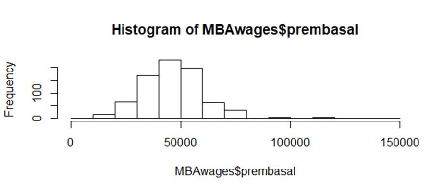
*prembasal; pre-MBA taker’s salaries

Figure 2 post-MBA workers' salaires distribution

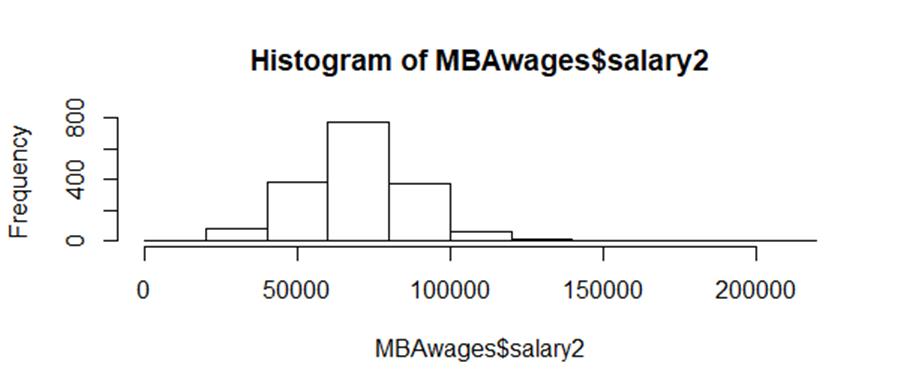
*salary2 ; post-MBA salaries.

 Apparently, it is roughly normal distribution. So we set on preliminary of hypotheses two-sample t-test.

 To find out whether the gap between the two means exists or not, the next step is to state the null hypotheses and alternative hypotheses in terms of  and . We would use Two-sided t-test due to the fact that we only have to check the equality of the two means. Assuming the null hypotheses is equality, where ; the pre-MBA salaries mean of the population is the same as the post-MBA salaries mean of the population. On the other hand, the alternative hypotheses is following ; their means are not equal. Significance level would be =0.05 as the criterion for this hypotheses test’s “statistical significance”. It will indicate whether the probability of null hypotheses is accepted or not. If the null hypotheses are more than the significance level, when α=0.05, it would not be rejected in this test because it might happen with more than 5% chances in the population. Otherwise, it will be rejected and we are 95% confident that the actual difference of salaries between pre-MBA workers and post-MBA workers could exist. Simplifying, we created these assumption values to test it.

 Key Parameters for the Analysis

 = Claimed value of mean salaries of pre-MBA

 = Claimed value of mean salaries of post-MBA

Null Hypotheses

There is no difference in the mean salaries between pre-MBA and post-MBA

Alternative Hypotheses

There is a difference in the mean salaries between pre-MBA and post-MBA

Results

 The output is taken by R with t-test. The p-value is <2.2e-16, fairly lower than significance level, which is 0.05. The p-value is the probability of our null hypotheses. In this case, it is shown that almost zero. “2.2e-16” is the smallest number that statistical software R can show. This analytic explanation is that we reject the null hypotheses that there is no difference between people who have an MBA and people who do not. Then, we could accept the alternative hypotheses that the difference in means is not equal to zero. According to the p-value, we are more than 99% confident that the difference of salaries, or alternative hypotheses, exists.

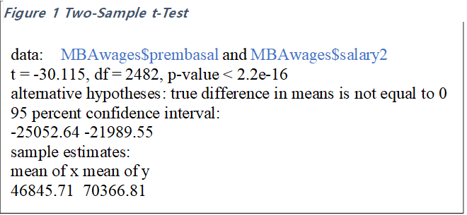 The confidence interval is -25052.64 to -21989.55, it is negative due to the fact that the post-MBA salaries() are subtracted from the pre-MBA salaries(). 95% of the salary gap between non-MBA taker and MBA taker is $-25,052 to $-21,989. This is evidence that proves roughly $23,000 is an annual ROI of an MBA program in general. Using statistic software R, we determine that our critical value’s interval for a two-sided test is +1.96 to -1.96. The difference between t-statistic value(-30) and interval(1.96) is tremendous. Repeatedly, this extreme data shows that the difference between the two means almost never happens. Estimates of the population are that the mean of pre-MBA salaries is $46,845.71 and post-MBA is $70,366.81. So, we calculate the salary difference is approximately $25,000.

Figure 4 Box plot of sample estimates mean

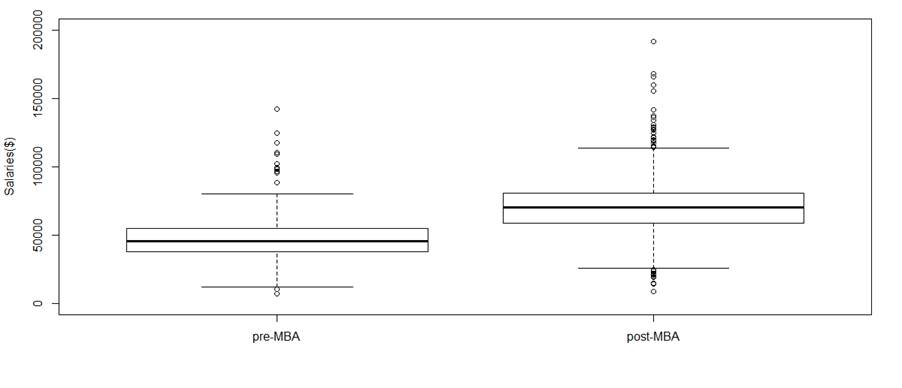
We can see the difference visually

Conclusion

 As we can see, the difference between t-statistic and critical value's interval is extremely huge. That is the fact that having no gap regarding MBA degree likely never happens, the p-value was 2.2e-16; the smallest number that R can show. On the other hand, an MBA program might be one of the factors contributing to higher salaries. The result of the sample estimates confirmed that there is approximately a $25,000 difference in non-MBA degree workers and the people with MBA degrees.

Figure 5 Confidence Interval of the t-Distribution

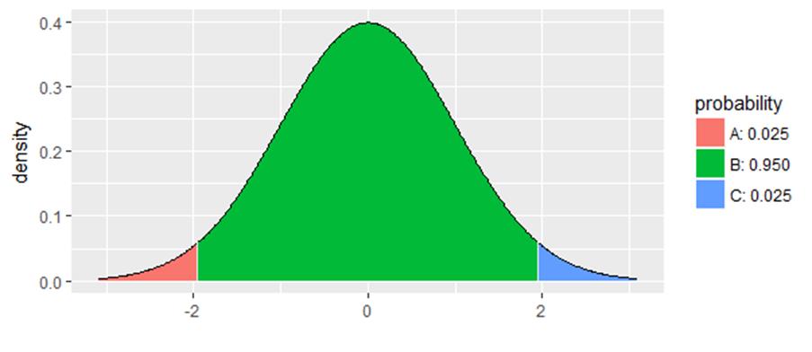
As a matter of fact, It is impossible to put critical value(-30) in this graph

 In closing, it is also worth mentioning that a pre-MBA taker could be looking forward to a $25,000 annual ROI after graduating from MBA business school by this fragmentary evidence.

 We ought not to conclude that MBA degrees caused an effect on salaries. In student t-test, it does not prove the causation, because it does not consider the potential effects from all other factors, such as working experience, industry etc.